Advanced Data Structure Types

Advanced data structures like trees, heaps, and hash tables keep data organized, enabling fast searches, and optimize systems for handling large datasets.

This is the second part of our series on Data Structure Types, where we delve into advanced structures like trees, graphs, and hash tables.

Consider a production system with linked data that works perfectly. What's the secret behind it all? Modern data structures keep everything clean, quick, and organized behind the scenes.

These structures determine if you can move data fast and handle millions of records, whether for real-time task prioritizing or sorting.

In this article, you will discover advanced data structure types and see how they can help change how hard data is handled.

Trees Data Structures

Picture trees: hierarchical structures of nodes linked by edges. Each node holds a value possibly pointing toward child nodes.

Atop sits a root node; nodes without children become leaves. Remember when you organized your files into folders and subfolders? That's like how trees structure data.

You'll find trees helpful in representing hierarchical relationships. They let you efficiently search, sort, and navigate structured data.

In this section, we'll briefly explore:

• Binary trees
• Binary search trees
• Balanced trees
• Heaps

Binary Tree

This time, each node of our trees branches into two paths: left and right. That's a binary tree for you!

Think of it like making decisions at every fork in a road—you choose left or right.

Binary trees are foundational in many search and sorting algorithms you might encounter.

Data Project from Physician Partners: Outliers Detection

Physician partners used this data project in the recruitment process of data scientists; check from here. You can see the dataset description below.

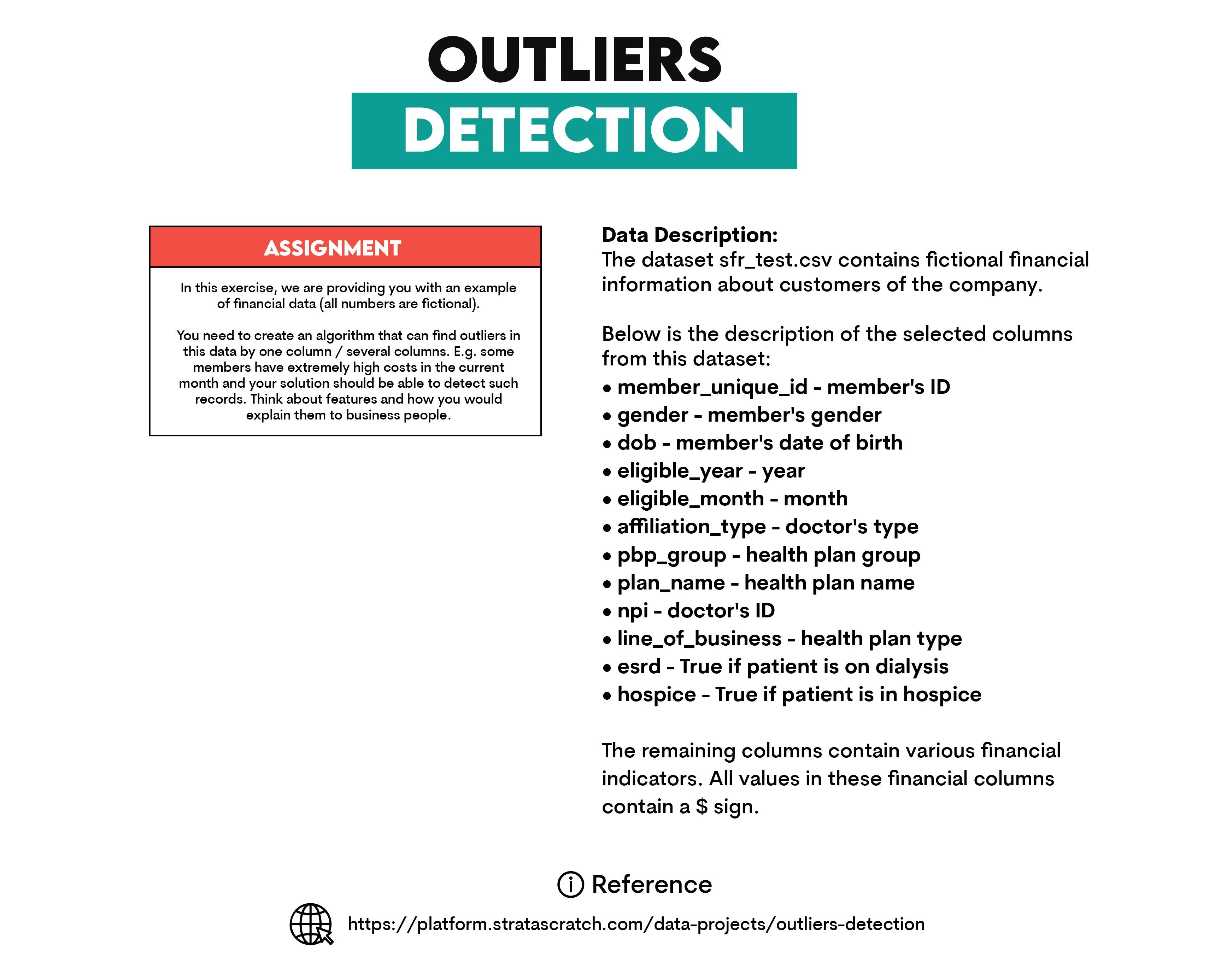
Before writing the code, let’s load the libraries in this article.

import heapq
import pandas as pd
import networkx as nx
import matplotlib.pyplot as plt

Let’s implement a binary tree in Python to store and traverse financial data like plan_premium? Here's how you can do it.

class Node:
    def __init__(self, data):
        self.data = data
        self.le ft = None
        self.right = None

class BinaryTree:
    def __init__(self):
        self.root = None
    def insert(self, data):
        if self.root is None:
            self.root = Node(data)
        else:
            self._insert_recursive(self.root, data)

    def _insert_recursive(self, current, data):
        if data < current.data:
            if current.left is None:
                current.left = Node(data)
            else:
                self._insert_recursive(current.left, data)
        else:
            if current.right is None:
                current.right = Node(data)
            else:
                self._insert_recursive(current.right, data)
    def inorder_traversal(self, node):
        if node:
            self.inorder_traversal(node.left)
            print(f"Plan Premium: ${node.data:.2f}")
            self.inorder_traversal(node.right)

binary_tree = BinaryTree()

for premium in plan_premiums[:5]:  # Limiting to the first 5 values
    binary_tree.insert(premium)

binary_tree.inorder_traversal(binary_tree.root)

Here is the output.

This simple code defines a binary tree and then scans the nodes in order to print them. The tree is divided by financial premiums in value, allowing lower values to be located on the left and higher ones on the right. Binary trees are still lovely when you want your data structure sorted for efficient search and traversal.

Binary Search Tree (BST)

In BST, all the nodes are in a particular order. It saves its children elements, so each has a lesser value than the parent on the left side and greater values on higher levels.

Explanation of the Code:

Here’s how to implement a binary search tree for handling financial data.

class Node:
    def __init__(self, data):
        self.data = data
        self.left = None
        self.right = None

class BinarySearchTree:
    def __init__(self):
        self.root = None

    def insert(self, data):
        if self.root is None:
            self.root = Node(data)
        else:
            self._insert_recursive(self.root, data)
    def _insert_recursive(self, current, data):
        if data < current.data:
            if current.left is None:
                current.left = Node(data)
            else:
                self._insert_recursive(current.left, data)
        else:
            if current.right is None:
                current.right = Node(data)
            else:
                self._insert_recursive(current.right, data)
    def search(self, data):
        return self._search_recursive(self.root, data)
    def _search_recursive(self, current, data):
        if current is None or current.data == data:
            return current
        if data < current.data:
            return self._search_recursive(current.left, data)
        return self._search_recursive(current.right, data)
    def inorder_traversal(self, node):
        if node:
            self.inorder_traversal(node.left)
            print(f"Plan Premium: ${node.data:.2f}")
            self.inorder_traversal(node.right)
bst = BinarySearchTree()

for premium in plan_premiums[:5]:  # Limiting to the first 5 values
    bst.insert(premium)

search_value = plan_premiums[2]  # Arbitrarily choosing one of the inserted values
result = bst.search(search_value)
if result:
    print(f"\nFound Plan Premium: ${result.data:.2f}")
else:
    print("\nPlan Premium not found.")

bst.inorder_traversal(bst.root)

Here is the output.

This code builds a binary tree and performs an in-order traversal to display the nodes. The tree organizes financial premiums by placing smaller values on the left and larger ones on the right.

Binary trees are particularly useful when you need a sorted structure for efficient searching and navigation.

Balanced Trees

Now, let’s imagine trees that cleverly keep their height minimal—that's what balanced trees do! They ensure that operations like searching, inserting, and deleting data stay efficient.

Examples? You might have heard of AVL trees or Red-Black trees. These trees automatically adjust themselves during insertions and deletions to remain balanced.

The height difference between left and right subtrees in balanced trees stays minimal, typically within one level. This property keeps operations efficient even in worst-case scenarios, so you get logarithmic time complexity.

Have you ever wondered how databases stay so quick? Balanced trees play a big role there! Maintaining a balanced structure is essential in systems where performance is critical, like databases and indexing systems.

Heaps

Heaps, specialized tree-based data structures, satisfy the heap property.

The parent node always stands greater than or equal to its children for a max-heap. Conversely, the parent node remains less than or equal to its offspring in a min-heap.

You'll find heaps widely used in priority queues and sorting algorithms.

Explanation of the Code:

Here’s how you can implement a min-heap using Python’s heapq module.

class MinHeap:
    def __init__(self):
        self.heap = []

    def insert(self, data):
        heapq.heappush(self.heap, data)

    def remove_min(self):
        if len(self.heap) > 0:
            return heapq.heappop(self.heap)
        else:
            return "Heap is empty."

    def display(self):
        print("Current Min-Heap:")
        for item in self.heap:
            print(f"Plan Premium: ${item:.2f}")
min_heap = MinHeap()

for premium in plan_premiums[:5]:  # Limiting to the first 5 values
    min_heap.insert(premium)

min_heap.display()

removed_premium = min_heap.remove_min()
print(f"\nRemoved Plan Premium: ${removed_premium:.2f}")
min_heap.display()

Here is the output.

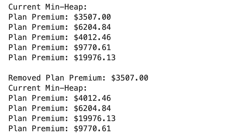
Using a min-heap, you consistently keep the smallest element at the root—perfect for tasks like quickly finding minimum values in datasets.

Heaps shine in algorithms like heap sort and efficiently managing dynamic priority queues.

Graphs Data Structures

Graphs are collections of nodes—also known as vertices—connected by edges. They model relationships in many domains, from social networks to recommendation systems.

Graphs are incredibly powerful tools enabling us to visualize and analyze complex relationships in ways difficult with other data structures.

Directed vs. Undirected Graphs

In a directed graph, edges have directions, indicating one-way relationships between nodes. For instance, in your dataset, you can visualize relationships between customers and doctors.

Each customer connects to their affiliated doctors, clearly demonstrating crucial connections for analyzing relationships within a healthcare system.

Explanation of the Code:

The following code creates a directed graph where nodes represent customers and doctors. Edges represent affiliations between them.

sample_data = data.head(20) 
G = nx.DiGraph()

customers = sample_data['member_unique_id'].unique()
doctors = sample_data['npi'].unique()

G.add_nodes_from(customers, type='Customer')
G.add_nodes_from(doctors, type='Doctor')

for _, row in sample_data.iterrows():
    G.add_edge(row['member_unique_id'], row['npi'])

plt.figure(figsize=(10, 8))
pos = nx.spring_layout(G, seed=42)  # Optimized layout for spacing
nx.draw(G, pos, with_labels=True, node_color='skyblue', node_size=700, font_size=10, font_weight='bold', edge_color='gray', arrows=True)
plt.title("Directed Graph: Customer to Doctor Affiliations")
plt.show()

Here is the output.

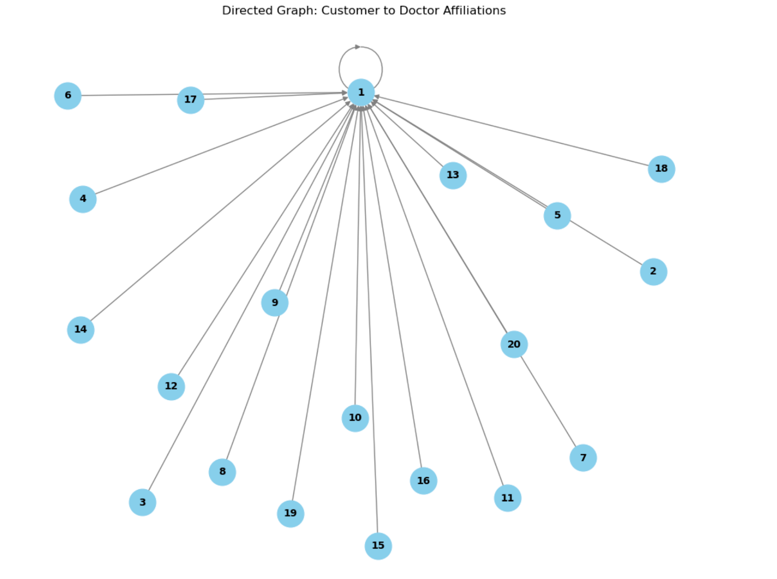
In this directed graph, customers are linked directly to their affiliated doctors. The layout optimizes connections, reducing overlap and making relationships easier for you to interpret.

These visualizations help you spot patterns and clusters. They allow you to analyze customer-doctor relationships and detect potential bottlenecks or key connections.

Weighted vs. Unweighted Graphs (With Dataset)

Weighted graphs assign weights on edges, often representing cost, distance, or other metrics. You might apply weighted graphs to represent financial relationships in your dataset. Each edge's weight corresponds to an economic indicator—perhaps the premium amounts customers pay to specific institutions.

Explanation of the Code:

We'll build a weighted graph where nodes represent customers and institutions. Edges represent financial transactions, with weights corresponding to plan_premium values.

sample_data = data.head(20) 
# Create a weighted graph
G_weighted = nx.DiGraph()

customers = sample_data['member_unique_id'].unique()
institutions = sample_data['plan_name'].unique()

G_weighted.add_nodes_from(customers, type='Customer')
G_weighted.add_nodes_from(institutions, type='Institution')

for _, row in sample_data.iterrows():
    # Convert plan premium to float and use it as the weight
    weight = float(row['plan_premium'].replace('$', '').replace(',', '')) if isinstance(row['plan_premium'], str) else 0
    G_weighted.add_edge(row['member_unique_id'], row['plan_name'], weight=weight)

plt.figure(figsize=(12, 10))
pos = nx.spring_layout(G_weighted, seed=42)  # Optimized layout for spacing
edges = G_weighted.edges(data=True)
weights = [edge[2]['weight'] / 1000 for edge in edges]  # Scaling weights for better visibility

nx.draw(G_weighted, pos, with_labels=True, node_color='lightgreen', node_size=800, font_size=10, font_weight='bold', edge_color='gray', width=weights, arrows=True)
plt.title("Weighted Graph: Customer to Institution Transactions (Plan Premium)")
plt.show()

Here is the output.

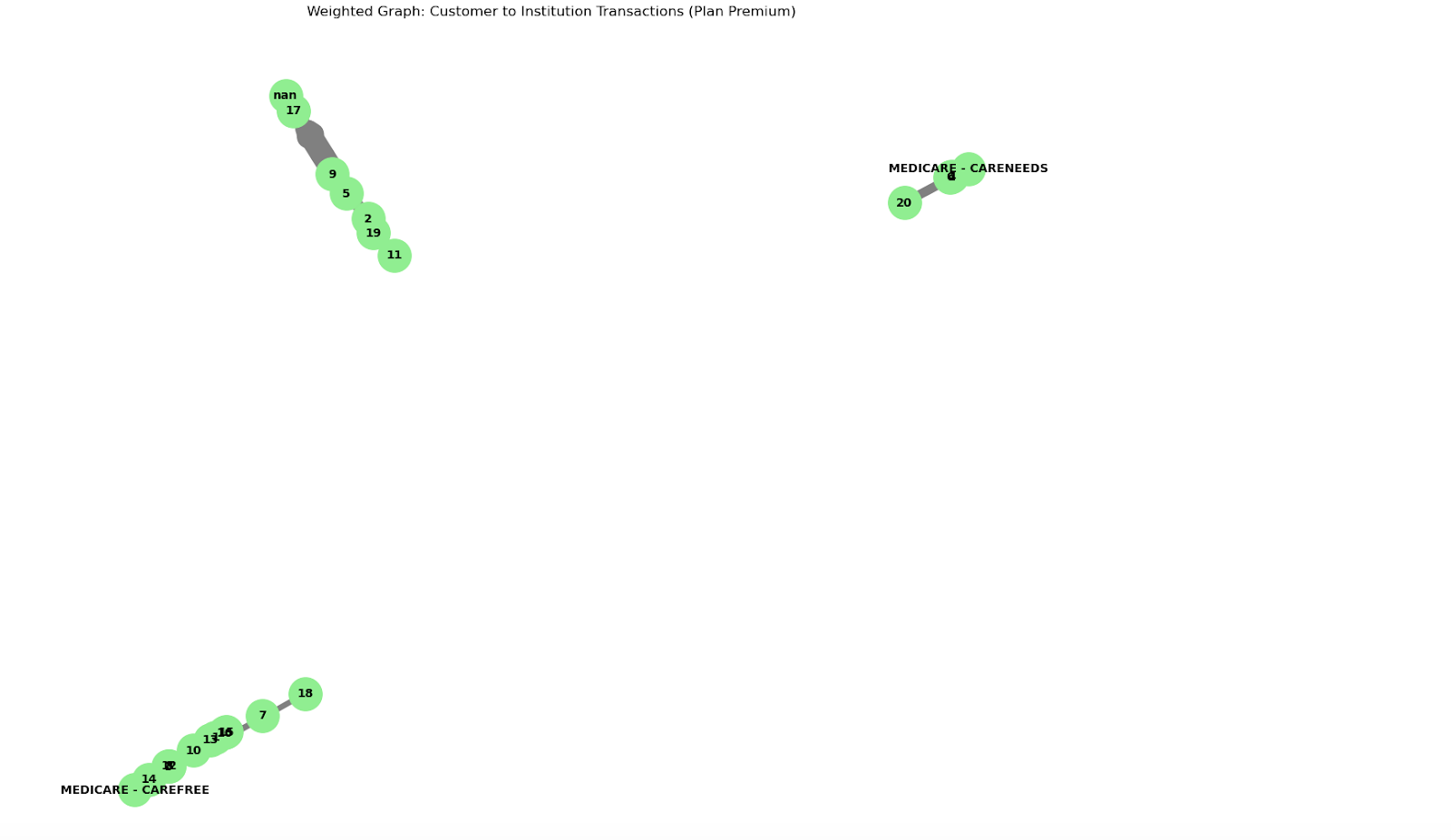
In this weighted graph, customers connect with institutions; edge weights represent plan_premium values.

Edge thickness increases with premium amounts, helping you visually spot relationships involving higher or lower transactions.

This visualization becomes valuable when analyzing revenue distribution or identifying high-value customers.

Cyclic vs. Acyclic Graphs (With Dataset)

A cyclic graph contains at least one cycle—a path that starts and ends at the same node. An acyclic graph lacks these cycles entirely.

Directed Acyclic Graphs (DAGs) prove especially useful in data science applications like task scheduling, dependency resolution, and data pipelines.

Explanation of the Code:

Here's how you can detect whether a graph contains cycles and visualize any that are found.

is_acyclic = nx.is_directed_acyclic_graph(G_weighted)

if is_acyclic:
    print("The graph is acyclic (DAG).")
else:
    print("The graph contains cycles.")

cycles = list(nx.simple_cycles(G_weighted))
if cycles:
    print(f"Cycles detected: {cycles}")
else:
    print("No cycles detected.")

Here is the output.

This code diligently checks whether a graph remains acyclic, carefully spotting any cycles lurking within.

In complex financial systems, unexpectedly finding cycles could reveal potential fraud, circular dependencies, or transaction loops needing further analysis.

DAGs become especially crucial in data pipelines.

They ensure tasks are processed in the correct order without accidentally causing infinite loops.

Hash Tables Data Structures

Hash tables map keys to values using a hash function. This function takes a key, produces a hash code, and then uses it as an index for storing the corresponding value.

Hash tables excel at operations like insertion, deletion, and lookup. They're incredibly efficient, making them ideal when you need quick access to data.

Insert

In hash tables, the insert operation efficiently stores key-value pairs. Imagine mapping customer IDs directly to their plan_premium values.

Explanation of the Code:

Curious about how to create a hash table in Python using a dictionary? Here's how you might store customer IDs as keys and plan_premium as values.

sample_data = data.head(20)  
hash_table = {}

for _, row in sample_data.iterrows():
    customer_id = row['member_unique_id']
    plan_premium = float(row['plan_premium'].replace('$', '').replace(',', '')) if isinstance(row['plan_premium'], str) else 0
    hash_table[customer_id] = plan_premium

print("Customer ID -> Plan Premium:")
for customer_id, premium in hash_table.items():
    print(f"{customer_id} -> ${premium:.2f}")

Here is the output.

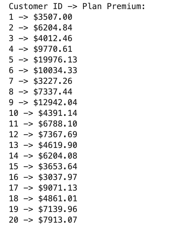
In this code, each customer ID cleverly maps to its plan_premium via a dictionary. This setup allows for quick lookups.

You can easily retrieve a customer's premium without painstakingly scanning the entire dataset. Hash tables become incredibly useful when you're dealing with large datasets where fast access is absolutely critical.

Delete

Removing entries in a hash table? It's as simple as deleting a key-value pair.

Explanation of the Code:

Here's how you can quickly implement a delete operation.

def delete_customer(hash_table, customer_id):
    if customer_id in hash_table:
        del hash_table[customer_id]
        print(f"Deleted customer {customer_id} from the hash table.")
    else:
        print(f"Customer {customer_id} not found in the hash table.")

customer_to_delete = sample_data.iloc[0]['member_unique_id']  delete_customer(hash_table, customer_to_delete)

print("\nUpdated Hash Table:")
for customer_id, premium in hash_table.items():
    print(f"{customer_id} -> ${premium:.2f}")

Here is the output.

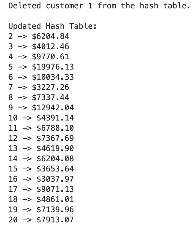
This code efficiently deletes a customer record based on the customer ID from the hash table.

Efficient deletion keeps your hash table current, which is crucial in applications like customer management systems where data needs frequent updates.

Search

The search operation retrieves the value linked to a specific key. In our scenario, you can quickly find the plan_premium for a particular customer ID.

Explanation of the Code:

Here’s how to implement the search functionality:

def search_customer(hash_table, customer_id):
    return hash_table.get(customer_id, "Customer not found")

customer_to_search = sample_data.iloc[1]['member_unique_id']  
premium = search_customer(hash_table, customer_to_search)
if isinstance(premium, float):
    print(f"Customer {customer_to_search} has a plan premium of ${premium:.2f}.")
else:
    print(premium)

Here is the output.

The search is simple and fast, taking an average of constant time. This feature is especially useful when swiftly retrieving customer information without scanning large datasets.

Conclusion

From hash tables to trees, these sophisticated data structures—the unsung heroes—keep our systems functioning without incident. Knowing when and how to apply these structures will significantly increase your efficiency in organizing hierarchical relationships, maintaining priority queues, or quickly searching a lot of data.